An Introduction to Bayesian Modeling

By Diego Marcano

One of the most powerful ideas that comes out of using the Bayesian statistics we've learned in class is the idea of Bayesian inference. One of the best ways to describe what Bayesian inference means is through an example.

You are looking for a place out to eat. After finding a place, you want to make sure that you won't waste your time and money so you go and read the reviews. The first review you reads "This place has amazing food!". The next set of reviews also have a similiar tone to them reasurring you that the restaurant might be a good choice after all...

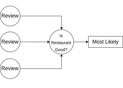
Fig. Using reviews to update our beliefs of a restaurant

This way of thinking is exactly what Bayesian inference is. The idea of simply updating your beliefs after considering new evidence.

We can try to leverage this way of thinking to create an algorithm that can use Bayesian inference in a wide variety of problems. One of the more straightforward algorithms is called the Naive Bayes Classifier. We're going to look at the inner workings of this algorithms by taking the example of classifying restaurant reviews.

Naive Bayes: A Straightforward Introduction to Bayesian Inference for Machine Learning

Naive Bayes is what is called a supervised learning algorithm. It takes in a sample dataset and uses that data to predict outcomes from data that it has never seen before. In our Example we're going to use a mock dataset that corresponds to positive and negative restaurant reviews. From this small set of data we will then predict wheter new reviews are positive or negative.

Here is the Outline of this page

1. Training Naive Bayes
2. Making predictions
3. Dealing with never before seen words
4. Pros and Cons of Naive Bayes
5. Naive Bayes Real World Scenario 4

1: Gather Dataset and Train The Classifier

The most important step in all of this is gathering our dataset. Our results can vary wildly depending on how good our data is. For this example I created a sample dataset to keep things simple.

Text	Label
simply loved it	1
this food was bad	0
really good food	1
terrible taste	0
this food good	1
loved taste	1
bad ambiance	0
i loved it so bad	1
i simply loved this good food	1
it wasn't good	0

Now we have a small dataset to train on. Every row corresponds to a review which has a label for either being a positive or negative review and a set of words that corresponds to the review.

(Notice how all words are lowercase and punctuation has been cut. This is an important step because we want to keep the data consistent when we train our model and when we predict on new data. Making everything lowercase and cutting punctuation makes it easier to learn from our data without chaning the end results.)

Now we can train our model. We imagine taking each and every review. Breaking it down by its words and adding that word to a bag of words. Making sure to what type of review each word came from. Doing this might lead to a bag of words that looks like this.

Word	Good Count	Bad Count
simply	2	0
loved	4	0
it	2	1
really	1	0
good	3	1
food	3	1
this	2	1
taste	1	1
i	2	0
so	1	0
bad	1	2
was	0	1
wasn't	0	1
ambiance	0	1
terrible	0	1
total counts	22	11
total reviews	6	4

We now have a table of how many times each word occurs in positive and negative reivews. With this, Naive Bayes is trained!

2: Calculating Basic Predictions

Fig. Is this good? Most Critics Agree.

Now the Naive-Bayes classifier has been trained. It contains a bag of words that we can use to begin classifying sentences into either:

positive (1) or negative (0) reviews.

Now lets calculate wether a new review is positive or negative. Assume we ask our model to predict whether the following sentence is a positive or negative review:

Food taste good

Not the most elegant review but a good example nonetheless.

Now our prediction follows the following steps

1. Process the data to make usable by the model
2. Find the probabilitiy of the sentence belonging to each label
3. Return the label from which the probabilitiy is the highest

First, we want to process this sentence such that we can use it in our naive bayes model. we split the sentence into its component words and make it a list of words

$Food$ $taste$ $good$ $\rightarrow food,taste,good$

Now from the list of words we ask the question, given a specific word, what is the probabilitiy that our review is positive or negative?

For each individual word, we simply look at the frequency each word pops up in our bag of words. A good visualization of this is making a histogram for the frequency of each word in our training set

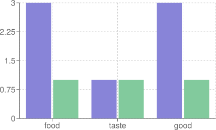
Lett's take a look at the word good

Given that we have the word good, what is the probability that our review is positive?

By Baye's rule this is

Looking at each term:

1. P(word =good | review = 1) -> number of times that the word "good" was in a training examlpe with label "1" divided by the number of times it was in the dataset

2. P(review =1 ) -> number of training examples that were labeled as "1" (positive reviews) divided by the total number of reviews

3. P(word = good) -> number of times that the word "good" shows up in our training data relative to all other words

Since we are dealing with a binary choice of labels we can rewrite the P(word = good) as

P(word = good) = P(word = good | review = 1)P(review = 1) + P(word = good| review = 0)P(review = 0)

From the probabilities listed above we can simply get the counts from our bag of word to calculate the probability of seeing a review that is positive given the word good

So with the word example this looks like

1. Look at bag of words to get the necessary frequencies

Word	Good Count	Bad Count
good	3	1
total counts	22	11
total reviews	6	4

2. Use the counts to calculate necessary probabilities

P(word =good | review = 1) = 3/4 = 0.75

P(review =1 ) = 22 / 33 = 0.67

P(word = good) = (0.67)(0.75) + (0.33)(0.25) = 0.58

3. Use Bayes Rule to calculate the probability a review is good

P(review = 1 | word = good) = ((0.67)(0.75))/0.58 = 0.86

We conclude that we have an 86 percent chance to have a positive review given just the word good

Now finding the probability of multiple words

We can easily find and label a one word review as either positive or negative but what do we do with our three word sentence review? We want to find the probability that a review is either positive or negative given a set number of words. This can be written as

There are multiple ways of finding this joint probability. One approach is by directly looking for any reviews that have the words food, taste, good, which can lead to a lot of difficulties. Either we have to keep looking through our training every time we want to make a prediction or we have to store every single possible word combination we run across. Even then we are not guaranteed to have seen a review with any arbitrary set of words we want.

Instead we can remember the idea of joint independent probabilities. The formula for two events A and B given that A and B are independent from each other is

In our case we can rewrite the probability of seeing each specific review as the product of the probabilities of seeing each individual word much like just looking at a one word review.

So

Now this is not entirely true. The fact that a word such as $good$ is in a review may indeed change the probability we see some other words such as $bad$ but in practice this assumption creates results that are very accurate even with small datasets.

This means that for Naive Bayes, we follow the following procedure

1. For every word in our review:
     a. Look up how many times the word appears for each label in our bag of words
     b. Use Baye's rule to calculate the probability shows up for each label (eg : P(word = "good" | label  = "positive review"))
     In our example we find the probability that we see each word in a positive and negative review. 

2. Take the product of the conditional probabilities of each word and multiply them together to find the probability that a sentence belongs to a specific label

The equation for this process can be written as

${\Large P(label = i | word1 \cap word_2 \cap ... \cap word_n ) =} {\Large \frac{ (\prod{k = 1}^{n} P(wordk | label = i ) ) \cdot P(label = i) }{\sum{label = i}^{m} ((\prod_{k = 1}^{n} P(word_k | label = i ) \cdot P(label = i) )} } $

Or the product of the probabilities of each word being in a specific label divided by the total probabilities each word belongs to all the labels

3: Dealing with never before seen words

As is the the current Classifier is very robust but still has one key drawback. To show this, we will look at the following review

Food was really bad

Not too bad. If we follow the previous steps then

1. Look at the bag of words for

Word	Positive Count	Negative Count
really	1	0
food	3	1
bad	1	2
was	0	1
total counts	22	11
total reviews	6	4

2. Calculate the probabilities

Here is were we go wrong. Looking at the words really and was we see that they each appeared 0 times in negative and positive reviews respectively. If we try to take their conditional probabilities we get

P(word =really | review = 0) = 0/1 = 0!

P(word =really | review = 1) = 1/0 = Oh no!

P(word =was | review = 1) = 0/1 = 0!

P(word =was | review = 1) = 1/0 = Oh no!

Having not seen a word in our dataset for all labels leads us to scenarios where we multiply and divide by 0! Depending on how we implement naive Bayes, this will either crash our program or return a 0 percent probability for all labels!

Because of this, we usually add to the classifier what is called a pseudocount. That is providing synthetic data to avoid these types of hiccups. What we do here is take every word in the bags of words, and add 1 to their total count

Word	Good Count	Bad Count
simply	2 +1	0+1
loved	4+1	0+1
it	2+1	1+1
really	1 +1	0+1
good	3+1	1+1
food	3+1	1+1
this	2+1	1+1
taste	1+1	1+1
i	2+1	0+1
so	1+1	0+1
bad	1+1	2+1
was	0+1	1+1
wasn't	0+1	1+1
ambiance	0+1	1+1
terrible	0+1	1+1
total counts	22+15	11+15
total reviews	6	4

Any number can be added but adding 1 is most commonly used in practice. By Adding these counts we no longer run into the problems of having 0 frequencies. The good thing is that adding these counts also does not impede the ability for the model to make inferences even if our dataset is small.

4: Pros and Cons of Naive Bayes

Naive Bayes is a widely known machine learning algorithm for classification problems. It is both fairly straightforward to understand and implement and can lead to quick results.

Overall one can categorize the pros and cons as such:

Pro's

• Straightforward to implement and change
• Very fast to train
• Very fast to tweak
• does not require very large datasets

Con's

• Diminishing returns on increasing dataset size
• Require's field expertise on words that one might ignore or not
• Limited if categorical data is not inherently independent

More modern machine learning methods such as convolutional neural networks (CNN) and reccurrent neural networks (RNN) do a much better job when given very large datasets. This does not mean that there is no space for Naive Bayes as it can serve as a very good initial explaratory model of the any given dataset.